By
Mark Stammers AMIMI
Introduction
I started writing this guide back in 2007, after about seven or eight years of using my digital storage oscilloscope (‘DSO’). The idea came to me as a way of challenging my understanding of the tool and to maybe help someone else, either choose a ‘scope’ or understand the one they were using, better.
I started in the motor industry in 1980 as an apprentice mechanic, for a franchised dealership. During this time it became quite clear to me that my passion was for the diagnostic side of the job. Towards the later part of the 1980’s, I started to see a significant development of electronics used on the cars, like ignition system management, petrol injection management, anti-lock braking systems, climate control, cruise control and much much more.
Part of my passion was finding methods to make diagnoses easier, quicker and more reliable. With the developments taking place and the problems arising, this was becoming ever more necessary.
Towards the end of the 1990’s, I had become more and more frustrated with the limitations of the manufacturers diagnostic tools, along with my own equipment. I decided the time to upgrade my own equipment had come. Firstly, my multimeter was to be replaced. I looked into what was available through the normal channels in the motor trade and felt disappointed. So I then looked into what was about, outside the normal. I spoke to an engineer at Fluke Industrial and discussed my needs. With his help, I decided upon a fairly ‘high-end’, ‘Industrial’ multimeter, as opposed to the dedicated ‘Automotive’ meter.
At that time, all the ‘Automotive’ meters were set up for ‘RPM’ measurements and dwell angles, for dealing with ‘points ignition’ and had pretty slow update rates. I wanted something which could measure frequency, duty cycle and pulse width and have fast update rates. Nowadays, of course, the ‘Automotive’ meters are much improved and more appropriate to modern systems, but at that time, they really were ‘behind the times’.
After some time familiarising myself with the instrument, it became apparent I had been missing out so much when it came to analysing the vehicle electronic systems, I knew I had to make the leap and go for an oscilloscope. I had, of course, been looking at ‘scopes, in the brochures, whilst investigating multimeters and had in mind one or two instruments, which seemed to have everything I thought I could use and understand. (I hadn’t used a proper oscilloscope since my college days and certainly not a digital storage scope, or DSO). However, after a lot more discussion with my friendly Fluke engineer, along with an incredible deal, I purchased a ‘high-end’ portable, (hand held), ‘Industrial’ Digital Oscilloscope.
Again it seemed that at that time any ‘Automotive’ instrument was just too slow and restricting for the modern and developing systems and so the ‘Industrial’ engineering world was where we needed to look.
When the new tool arrived, I read the hand book from cover to cover and proceeded to do nothing but ‘play’ with it. (Still the best advice for any new equipment). I would connect it up to just about every vehicle that passed through my work bay, plus a few in the bay next door.
I was fascinated by the effects of looking at voltage at different speeds and noticing how different it could be and what it would reveal. However, I stayed away from making any diagnostic decisions with it for quite some time. I really wanted to get confident using it before I would rely on the evidence it would present me with. You really need to learn to read the signals and no what is good and bad. Whenever I would get the chance, I would take a sample of a known good case and also a known bad sample. I still do that today and will continue to do so.
Understanding the Instrument
I think a good start to understanding the ‘DSO’, is to start by understanding the digital multimeter or ‘DMM’, specifically the voltage measurement side or ‘DVM’.
We’ll also look at some things that perhaps you had not even thought about. They may help you either choose a ‘scope or better understand the one you have.
‘If we have a look at the DVM and what it does, we start to understand why we need to start using a DSO’.
The Digital Voltmeter (DVM)
A digital voltmeter or DVM displays either a percentage of the maximum voltage present or the maximum voltage present on a signal, depending whether the signal is a stable direct current signal or an alternating current signal. What you get to see is determined by the meter’s capability and is not always the full picture. In the case of a straight forward DC (direct current) voltage, like a battery power supply to a relay, this is not a problem. But if the voltage switches from 12v to 0v quickly, like a pulsed supply to a solenoid, then you’ll only see part of the signal.
This is particularly noticeable when measuring AC (alternating current) voltage signals, like speed sensors or digital DC signals, like a camshaft sensor. If you use a basic ‘average responding’ meter, you will see less voltage than you will see with a ‘True RMS’ * meter. This was one of the factors I noticed after the purchase of my new ‘True RMS’ multimeter compared to my old one.
Although the voltage value, may not be so significant as such, the ability to capture the rapid changes, may be important.
*A ‘True RMS’ (Route Mean Square) meter will display a higher voltage for a non-sinusoidal wave, such as a square wave, than an ‘average responding’ meter.
Let’s see if I can demonstrate:
A car comes into your workshop with a trouble code P0340, camshaft sensor malfunction. You want to check the sensor for correct operation. It’s a 3 wire ‘hall effect’ sensor. You start the car and then you back-probe the wires going into the sensor. You find a nice 5 volts on pin 1, 0 volts on pin 3 and about 2.3 volts on pin 2. Why is there 2.3 volts present? Surely it should be either 0 volts or 5 volts switching quickly. Well that’s the phenomena of the DVM. The meter can only display an average reading. Depending on how fast your meter can react, will determine the exact reading you see, but the relationship between the amount of time the signal is high against that of the signal low (duty cycle), will determine the voltage display above or below the halfway mark.
The example below illustrates what I’m trying to get across.
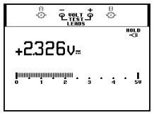
This image is the screen capture of a ‘True RMS’ voltmeter, measuring a camshaft position sensor, with the engine running. As you can see it reads just under half of the total 5 volt signal that should be seen.
This image shows the same camshaft sensor signal as in the previous image. As you can see the signal plainly switches from 0 volts to 5 volts.
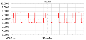
The average duty cycle on the low side of the signal is calculated at approximately 51%, therefore the average voltage will be under half, which is shown in the meter reading, although the reading is not necessarily accurate due to speed limitations of the meter.
Note: Low quality multimeters may only have a display update rate of 2 to 3 times per second, whereas higher-end meters may have update rates of 4 to 5 times per second. If your meter has an analogue bar graph display as well as the digital reading, like the one shown, the bar graph will react much quicker to a signal change, typically around 40 times a second, and consequently very useful when looking for those intermittent faults or glitches.
Don’t get me wrong; a good DMM, is still ‘worth its weight in gold’ as a diagnostic tool, and is still my most frequently used tool to date.
The Digital Storage Oscilloscope or ‘DSO’
An oscilloscope is an instrument that samples voltage * over a designated, but user defined, time frame. That voltage is then displayed on a screen for you in the form of a graph. It really is a case of ‘pictures versus numbers’. This means you instantly get to see more of, or indeed, all of the actual voltage and therefore all that is going on. Typically a ‘scope is much faster than a multimeter. What I mean is; the instrument samples the voltage signal and displays it much quicker than a DMM **.
The digital storage oscilloscope stores samples, before displaying them. This is the difference between a conventional CRT (Cathode Ray Tube), or analogue type ‘scope and a DSO. This does of course mean that typically the DSO is slower than the CRT ‘scope, but like all things digital, the DSO is more versatile. Storage is probably the main benefit. Nowadays, with super fast processors and huge capacity hard disks, the speed issue is negligible and in my opinion outweighed by the versatility of digital, for automotive work.
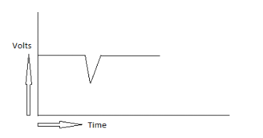
If you look at the image below, you can see the basic layout of a ‘scope. You can easily see how useful it can be for seeing those quick changes in voltage, rather than trying to catch your DVM display.
* Please don’t be put off by the fact that the oscilloscope samples voltage, when you may want a tool to measure other mediums such as current, temperature or pressure. Transducers can be used to convert these inputs into voltage, but we’ll talk about these later.
** A fairly low cost ‘automotive’ scope may have a bandwidth of approximately 300 to 400kHz, whereas a ‘high end’ DMM may only have as much as 100kHz. (I’ll explain bandwidth in the next section).
Basic explanations for instrument specifications
‘Bandwidth’
(specified in Hz/kHz/MHz/GHz) determines the capability of the instrument to measure a repetitive signal. For rapidly changing signals you need an instrument that can keep up. As a rule, in engineering terms, you need to specify a bandwidth approximately five times the maximum frequency you are likely to measure. Remember the more the bandwidth the better chance of capturing the signal accurately. But don’t pay for more than you need.
To explain the point a little more;
Say you have an oscilloscope with a maximum bandwidth of 100 kHz, a little unlikely these days I know, but I have seen a tool with less and it’s useful as an illustration. You want to measure a signal that has a frequency of 500 kHz; then you would not be surprised if the signal was not accurate or missing some detail. The instrument could not possibly keep up. See Figure 0.1
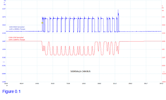
In Figure 0.1 you will see a sample of a CAN high speed bus. The CAN High signal (blue) is sampled at full bandwidth (20MHz) and the CAN Low signal (red) is restricted down to 100kHz.
(The sample was captured at 20MHz and filtered down to 100kHz for display purposes. Although it is not a true bandwidth limited sample, it is representative of a bandwidth limited capture).
It illustrates how the detail of the ‘mirror’ image signal, lacks representation. This is the result of insufficient bandwidth available to keep up with the signal speed.
‘Sample rate’
(specified in S/s / KS/s MS/s / GS/s) has a similar importance to bandwidth. It relates to how frequently the ‘tool’ takes ‘snap-shots’ or samples of the signal per second. The higher the sample rate the better the resolution, or detail, of the image displayed for you. (The tool takes sample point or dots and joins them up. The more dots taken, the better the ability to represent the signal). Consequently the more likely you’ll not miss important details. You may notice that when you select a long sample time base, you will miss information that you would have seen if you selected a shorter time base. That’s because the sample interval rate changes at different time base settings. On some instruments the maximum sample rate is only achieved at faster time bases; refer to your ‘scope manual.
The newer PC based ‘scopes, generally have configurable sample rates, whereas some of the dedicated instruments may have pre-defined rates. This may be something to be aware of when choosing a tool. The image below illustrates the sampling effects.
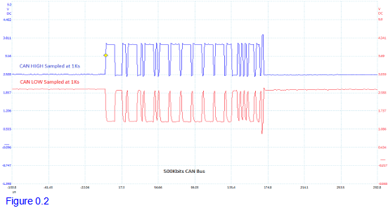
In Figure 0.2 the same High speed CAN signal as in Figure 0.1, is shown with the sample rate reduced to 1Ks, (1,000 samples, compared to 20,000 samples in the previous). You will notice there is reduced clarity of detail from the previous full bandwidth signal, (blue signal). Notice how the corners are not so square. This is because the sample interval is much larger, not so many dots to join up.
‘Memory Buffer or Record Length’
(specified in number of samples or points) refers to the amount of sample points, which can be stored in memory. The larger the number the more detail can be stored and recalled for zooming in on your stored waveform, for detailed analysis. This is especially noticeable for long waveform samples. The maximum specification for the memory, is usually split across all active channels, unless specified otherwise. High end stand alone, industrial DSO’s may have fairly large memory lengths, which may be available on all channels, but traditionally PC based DSO’s will have much larger capacity, even if splitting across all active channels.
‘Input Digitisers’
are the devices that convert the input signal (voltage) into a digital signal, of which can then be manipulated, stored and displayed by the tool. Ideally there would be one digitiser per channel, but you will find that is only on the ‘high end’ tools. If the ‘scope has only one input digitiser, then the tool has to swap or ‘chop’ from one channel to the other, sampling the signal on one channel then the other and so on. On some low-end ‘scopes this is very noticeable because at the faster time bases the ‘scope may only be able to measure on one channel, or it may reduce the bandwidth even further. Certainly the better quality scopes that use single digitisers manage this task perfectly well, so don’t let that put you off. Even so, the compromise is still noticeable in that, the sample rates may change when multiple channels are being used.
‘Isolated Floating Inputs’
relates to the type of input connection available for the signal ground. Similar to the input digitiser issue, usually only the ‘high end’ ‘scopes will have this feature and possibly only if the tool is portable. If the ‘scope doesn’t have isolated inputs, then it will share a ‘common’ ground input. This means that all the channels are linked to the ground connection, internally. This is fine if you want to measure multiple signals that all use a common ground. But some sensors may have, what is known as, ‘floating ground’. This means that their circuit is isolated from the main electrical circuit. An inductive or variable reluctance sensor (VRS), is a common example of this. Let’s say you want to measure something like an inductive engine speed sensor, which has a floating ground, and a camshaft hall effect sensor, which uses a common chassis ground, using two channels at the same time and you don’t have independent isolated inputs, then you will only measure half of the amplitude/voltage level of the engine speed sensor. In most cases, this is fine, as you probably only want to see that the sensor generates a voltage and that it represents speed and position. If you need to see the full voltage capability of the sensor, then you will need to measure across both sides of the sensor with one channel only. A ‘scope with isolated floating inputs, allows multiple channels to measure multiple signal types at the same time. As before, don’t get too worried about this, because there are ways of getting round that problem, but it is something to consider.
‘Attenuation’
relates to the voltage input ratio. The oscilloscope is a delicate instrument and should be protected from very high voltages. If the connection cables have an input ratio of 1:1, then whatever the level of voltage you measure will be passed directly into the scope. This is OK if the voltage is fairly low. You must know what the maximum input voltage of your ‘scope is and what the maximum voltage of your source is likely to be. If you want to connect to an ignition primary circuit, then you must expect voltages in the range of 400 volts. This may be too high for most ‘scopes and so that voltage needs to be reduced. This is done by ‘attenuation’. The norm’ would be around 10:1 or 20:1, depending on the tool’s protection level, although there are cases for 100:1 etc.
A 10:1 attenuator will step the voltage level from 400 volts to 40 volts. It is usually fitted to the input port between the test lead and the tool, or it maybe integrated into the test lead. Some leads have selectable attenuation.
‘Coupling’
refers to which portion of the voltage signal the instrument displays, either AC or DC. If you choose DC coupling, then you will see all of the voltage available, but if you choose AC coupling, then you will only see the AC portion of the signal, as the tool will remove the DC ‘off-set’. An example of this use maybe if you want to look at AC ripple created by an alternator, as the ripple will be a small amount at the top of the voltage output and so your screen will be taken up by 12 to 14 volts, when you are only interested in that little bit. If you select AC coupling, the screen will only show the ripple and so you can display much more of that signal.
There will be more about AC coupling further in the guide.
‘Triggering’
is a device used within the ‘scope to enable a signal to be displayed when and where you want it on the screen. If you set up a trigger, then you can stabilise the signal and concentrate the event right in the middle of the screen, if you wish. There are a number of trigger types employed and once again determined by the tool’s capabilities.
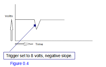
Edge triggering is a common trigger type and is used when the signal presents an edge, like an injector or ignition event. You can choose to trigger the ‘scope on either a rising or falling edge, by selecting a positive slope or a negative slope. Again you will need to check your ‘scope’s instruction for details on triggering, as they can use different terminology for each type. You may be able to set triggers for different pulse width intervals, or for specific signal conditions or complexities, or for a single shot display, so that the screen stops after it has seen one trigger event, and so on. The usefulness of such a device comes into it’s own when looking for an intermittent fault, like a ‘drop out’. Imagine you had set your ‘scope up with a ‘single shot on trigger’, with a voltage level of about 8 volts negative slope, connected to a fuel pump relay power supply. You could then just leave the tool monitoring the supply, whilst you drive the car or just leave it running and if the fault occurred, you would capture it.
Lets have a look in Figure 0.4, below.
‘BNC’ (Bayonet Neill Concelman) / ‘Banana’
refers to the input probe/test lead connection method.
The BNC connector is a single ‘quick’ connect/disconnect high frequency connection. Signal positive is carried in the centre pin and the ground is cased around it. It is, typically, used with a ‘Coax’ type cable.
Banana plug connection, usually 4mm is the standard method of connection for multi-meters, but is also used on some Digital Oscilloscopes.
Using the Oscilloscope
Most of the following examples are based on using a Fluke 190 series Scopemeter, your ‘scope may differ in set-up but the basic principles should be the same. Remember to check your ‘scopes input voltage limit and add attenuation as appropriate, before making any measurements.
First we’ll measure something nice and simple: A battery volt drop measurement.
Set the instrument to read DC voltage, then set the amplitude and time base to the following:-
Note: that where I state voltage or time per division, I am basing that on the ‘scope set-up. You may want to convert that to total screen voltage and total screen time.
-Channel A – Amplitude: 5v/div
-Channel B – Amplitude:500mV/div
-Time base: 1 sec/div
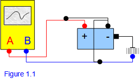
Connect channel A across vehicle battery:
(See figure 1.1)
-Signal probe to the positive
-Ground lead to the negative
Connect channel B to engine ground:
-Signal probe to engine block (Main earth)
-Ground lead to battery negative post.
(Remember; if your ‘scope uses a common input ground, you don’t need to connect channel B to ground).
Leave the ‘trigger setting’ off, if applicable, (we’ll cover ‘triggers’ later).
When you are ready, wait for the signal to start running from the left side of the screen, switch on the ignition and then start the engine.

When the signal reaches the far right side of the screen, press the hold button. You now have a capture of the battery performance and charging status along with the battery ground condition under load.
(See figure 1.2)
This is an essential test to start your diagnostic procedures when looking for those strange running faults or spurious fault code flagging.
I found this to be a very useful test that is really easy to do and carries a great deal of diagnostic value. Not only do you instantly see the integrity of the battery, you also see the performance of the ground cabling and ground connection and this is so easily over looked.
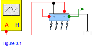
One of the first things I tried testing, when I purchased my ‘scope, was an ignition primary signal. So that’s what we’ll measure next; an ignition primary pattern.
Set the instrument as follows:
Warning: this measurement will be sampling voltages in excess of 400 volts.
-Channel A – Amplitude: 20v/div
-Time base: 1ms/div
Connect channel A as follows:
-Signal probe to the ignition coil
negative or trigger side.
-Ground lead to battery negative.
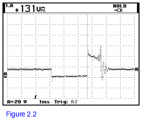
(See figure 2.1)

Once again, we’re going to leave the trigger function out of play. When you’re ready, start the engine and look at the screen. You should now be looking at the ignition primary pattern. (See figure 2.2)
If you don’t see the image, it is probably ‘zipping’ by too quickly to see, so try capturing it by pausing the screen as it goes by. You may need to keep trying until you catch it.
This will show why using the trigger function helps.
(For a detailed description of the waveforms shown, see the reference section).
That has seen how to make simple checks and signal acquisitions, but maybe it’s time to look at using the tool’s ‘Trigger’ function, as I’m sure you will have noticed that using the fast time base to look at a signal in detail, proved to be difficult and not very helpful.
Your ‘scope will probably have an automatic trigger function, but hopefully a manual option is available. Automatic is OK whilst starting to look at signals, especially if you’re unsure what the signal should look like, but manually setting the trigger point will allow you to choose when and where to start looking at the waveform. This makes much better use of the instrument. Remember though; you need to know what you are looking for before you can set a trigger function.
We’ll start by making the same measurement as we did in figure 1.2. This time though we’ll set the trigger point to acquire the signal without waiting for the screen to be in the right place.
For this particular acquisition, I have set the ‘trigger’ point to the following:
-Edge triggering, channel A
-Negative slope
-Level set at 10.2 volts
-Single shot option
All other settings are the same as in figure 1.2.

Now start the engine. You can see, in figure 3.0, that the instrument has waited until channel A sees a signal of less than 10.2 volts, (the voltage drop during cranking). At that point, it starts displaying the signal trace for the duration of the screen, including the signal prior to the trigger point. Because it is set with a single shot function, the signal will stop at the end of the screen. This means you don’t have to stop the screen.
Hopefully you found that easy, and it has made really efficient use of the tool. If your ‘scope allows you to save the set-up, then you can quickly recall it and use it again, without even thinking about it. This means that you can make many captures with the same settings and so build your library of experience, getting to know what is good and bad quickly and easily.
Now because that was sampling a long time base signal, it was not so important to get the trigger right. But if you want to sample a fast signal, it becomes much more important, as was seen in the primary ignition signal we tried earlier.
But what happens if you’re not sure where to trigger the ‘scope? You’re not sure what a particular signal should even look like, or maybe the signal you want to look at may have a problem and won’t trigger off your known set up.
So I think we’ll try going after an ignition primary signal as in figure 2.2, except we’ll imagine we don’t know what to expect.
In this exercise, we’ll show the ignition primary signal captured with the ‘scope, but with the view to not knowing where to trigger the instrument.
If we take the view that we know roughly what the signal should be in relation to time and voltage, we’ll set the scope as follows:
-Channel A – Amplitude: 20v/div
-Time base: 20ms/div
-Signal probe to the ignition coil negative or trigger side.
-Ground lead to battery negative.
See figure 3.1
Now when you run the engine, you should definitely see something.
You can see in figure 3.2, that I have held the screen shot, capturing three ignition events. From this screen capture you can get some idea of what the signal is like.
With some ‘scopes this may well be enough, especially if the instrument has a deep enough memory and allows you to zoom in significantly. But for a dynamic analysis this screen would not be good enough.
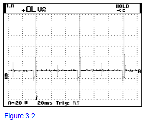
You would definitely want to see a much more detailed capture in-view.
So now we’ll adjust the channel settings to the following:
-Channel A – Amplitude: 20v/div
-Timebase 1ms/div
Now set the trigger function to the following:
-Edge triggering
-Positive slope
-Trigger position: approx. 60 volts and placed in the middle of the screen
-Free run mode or repeat on trigger
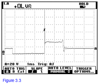
So, in figure 3.3 you can now see a much better view of the ignition primary signal, which will allow you to make a true analysis of what the ignition system is doing.
You may wish to play around with the trigger point to suit your tool and the particular system you are testing. This may be where bandwidth will play a part, as you may find the ‘scope triggers off of some high frequency signals present on the circuit. I’ll try and demonstrate.
When you first start using your ‘scope, you may become confused by the signals you see. I remember the first time I connected my, high speed ‘scope, to an engine temperature sensor and seeing kilovolts appear on the screen, with signals jumping up and down. What I was seeing, was the tool’s ‘auto’ detect function. The maximum bandwidth capability of the tool was 200MHz (200 million time per second), which meant it was capable of sampling really high frequency signals, and those signals were present for around 20 to 50 nanoseconds (1 nanosecond = 1 billionth of a second) and probably generated by the ignition system.
So what I was witnessing was the tool triggering off voltages present for such a short period of time, that they would have no influence on the operation of the sensor. But it did illustrate the need to gain experience in sampling signals that are normal, because it is not always what you might think.
It is also why you need to understand the tool and it’s capabilities, before you rely on it.
If you look at figure 3.4 you can see a signal glitch half way between the two ignition patterns.
In fact it is precisely 180 degrees between the two events and is caused by the opposite ignition channel interfering with the ignition circuit. It is quite normal, as you will get to see.
Now imagine if you set the trigger voltage to below 47 volts. You would be capturing all events that contain an edge within that amplitude. That maybe something you want to do, but equally it may detract from what you want to concentrate on.
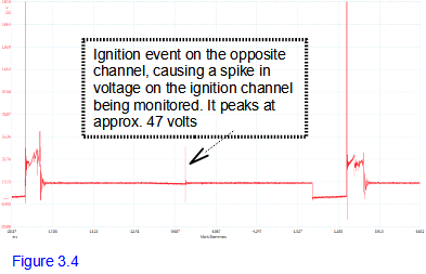
The signal in figure 3.4 illustrates what I am explaining, in that there are present some voltages for very short periods, which you might not of thought possible. The peak voltage of that glitch was present for only 35 nanoseconds.
You can imagine how that could be very distracting.
Now let’s take a look at ‘AC’ and ‘DC’ coupling, because I found it to be such a useful tool.
The example I’m going to use is the most common use of ‘AC’ coupling and used in every day diagnosis.
For your reference, all the ‘scope traces shown so far are ‘DC’ coupled signals. This is because we are measuring the entire voltage signal. In the example we are going to use next, we are only interested in the ‘AC’ portion of the voltage.
If you are not familiar with this expression, then I’ll try and explain in simple terms.
An alternator produces AC voltage, (alternating current), which is rectified by a series of diodes into ‘DC’ voltage, (direct current), which is stored in the vehicle battery.
Even a really good alternator will not rectify all the AC voltage, therefore if we look carefully at the charging voltage we can see what AC is left over. We can even see if a diode has failed. But like all these signals, you need to get use to them before you can identify a failure.
Set the instrument as follows:
Connect the probes as follows:
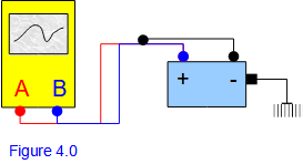
-Channel A red probe to battery positive
-Black probe to battery negative
-Channel B blue probe to battery positive
-Black probe to battery negative. See figure 4.0
-Channel A amplitude: 50mv/div
-Channel ‘AC’ coupled
-Time base: 2ms/div
-Channel B amplitude: 5 volts/div
-Channel B ‘DC’ coupled
-Set the trigger to positive edge at approximately 50mv on channel A
Please note:
It is more accurate to connect the scope probes directly to the BAT+ post on the alternator. But sometimes that’s really difficult to access.
However, there is sometimes an advantage to learning the values at the battery, as it can also demonstrate the ‘smoothing’ effect of a good battery. The detailed description in the reference section will demonstrate this.
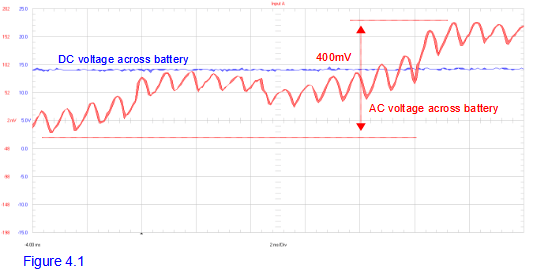
Figure 4.1 illustrates the AC content present on top of the DC voltage. The 400mV peak to peak, is an acceptable value for a good working system. More importantly the waveform shows no deformities, illustrating the integrity of the charging system, including the diode pack.
We will see more detail in the reference section.
This technique can be utilised in many cases where you are interested in the repeating cycle of a signal only. It can be used for looking at the detail portion of a manifold pressure sensor, showing the operation of intake valves and cylinder balance. So once again, the usefulness of a DSO is never to be under estimated.
I have found I don’t use this function so much with my later generation PC based oscilloscope, as it has so much memory and sampling depth. It will capture all of the signal and you can still zoom in on the smallest of details. Even so, when checking for AC content signals only, this technique is perfect and if your scope does not have such a large memory, the AC coupling will allow you to just concentrate on the bit you want to see.
That has probably given you an insight into the basics of setting up and using your oscilloscope efficiently. However there is much more available when you add some accessories to your kit.
Accessories
As with your multimeter, your ‘scope will only be useful if you can connect it to the things you want to test.
You need a good variety of probes and clips, because if you can’t connect securely to the subject, then you can’t analyse it.
One of the first problems I came up against with my ‘scope, was that it was equipped with ‘industrial’ electronics ‘scope probes’. Although I could use them, they were not brilliant for automotive work and I found myself making up adaptors to suit my needs.
I determined you really want test leads with 4mm banana ends, so that you can share your DMM accessories.
Among the first accessories you need to think about, are straight forward voltage sampling probes. Probably my most frequently used probes are the ‘back-pin probes’. These probes are very thin, but strong and flexible and allow you to slip past weather seals in the harness connectors. They allow you to access the terminal, without damaging any part of the connector, whilst still connected to whatever component you are testing. That’s the best way to test, as it keeps the circuit under load. This type of probe, and there are many variations available, are probably one of the most useful probes to invest in. You might have to try out some different ones before finding the one that best suits your needs. These come with 4mm banana socket and so easily interchange with test leads and generally these probes are inexpensive.
I use these every day with, both my ‘scope and my multimeter.
Once you start looking at 4mm banana test probes and clips, you will see there are a mass of choices available, so make good use of them and find the one’s that make the job as easy as possible.
As I mentioned earlier, voltage is not the only thing you can measure with your ‘scope. With the introduction of transducers, you can measure current, pressure, temperature, vibration, noise and so on..
The first transducer accessory I purchased, was an amp clamp. I highly recommend it, if you don’t already have one. This accessory will give you the ability to sample a component operation as if in 3D. Straight forward voltage tells you so much, but with the addition of current, you can really see if the component is actually consuming energy. Sometimes that evidence is completely obvious, but sometimes not so. Also it may allow you to determine a particular action of it’s operation. We’ll discuss this later in the guide.
As with all the accessories, there are many different varieties available consisting of different operating ranges, different jaw sizes etc. You need to select the most suitable for your needs.
Voltage and current sampling probes are a must for your basic DSO kit. We’ll see how they can be used in the next part of the guide. It will show the use of many different transducers, including low current and high current clamps and pressure transducers.
With the ever increasing availability of accessories, the only limitations of the DSO is your imagination.
