Engine System Sensors

Mass Air Flow sensors.

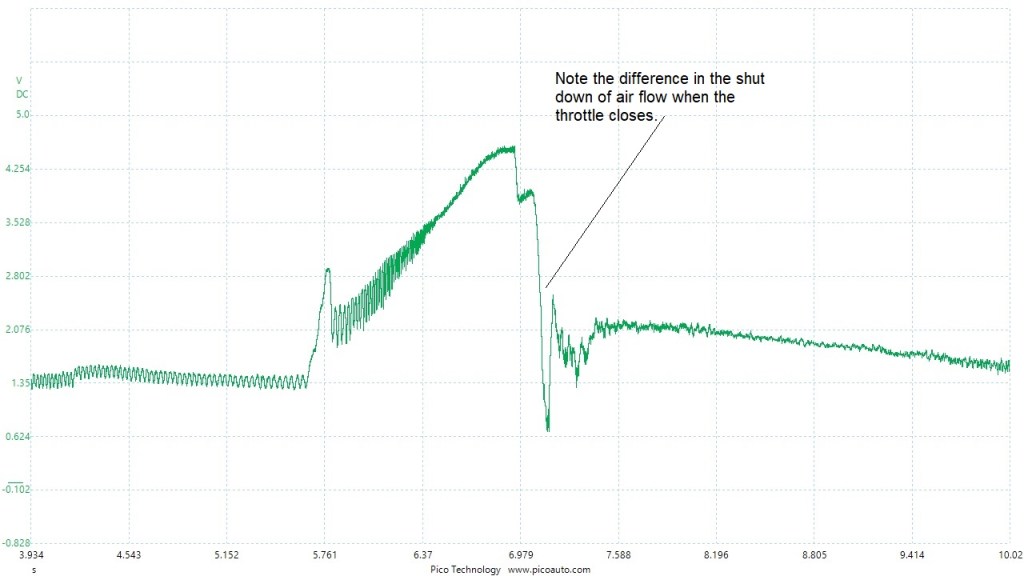
This first image, represents a naturally aspirated petrol engine mass air flow meter (MAF). It is of the hot film type, which is a modification of the hot wire type of sensor.

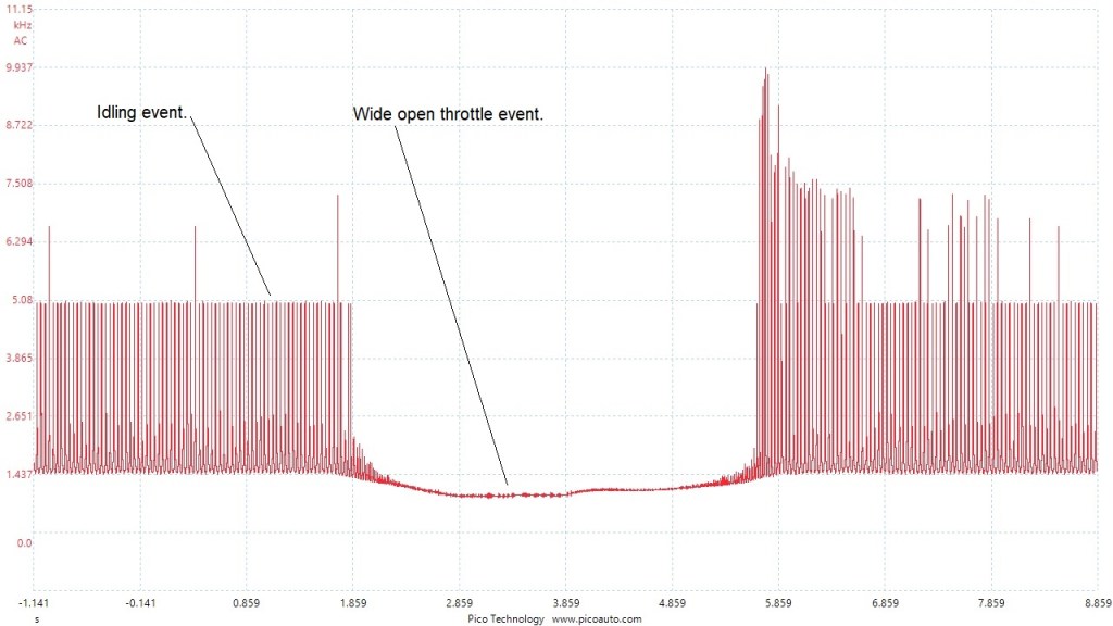
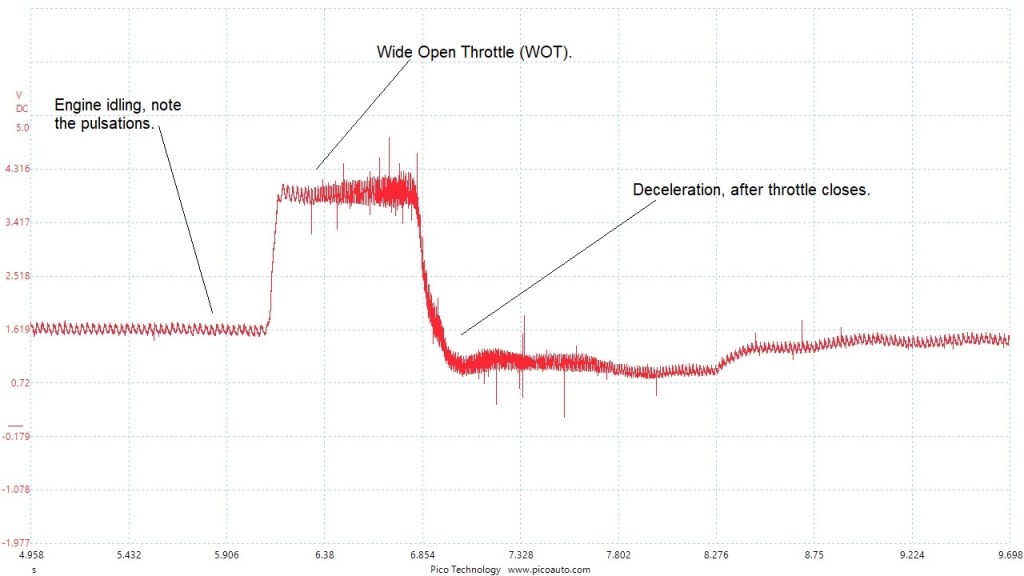
This capture was taken whilst idling, followed by a wide open throttle event or snap throttle.

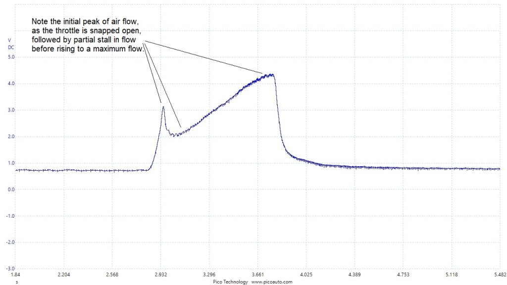
This is a fairly typical pattern of a good working MAF sensor and makes for a good quick test for maximum output. Usually, if you get the normal maximum output for a particular sensor, then it is probably good.

I very often do a quick test with my DVM, to see what the maximum output voltage reaches. This maybe useful for finding a bad responding meter, but it does not prove a good meter.

This is why you really need to get use to just breaking out the scope.

This sample shows a maximum output voltage of 4.3 volts, which generally is a good sign for a MAF.

But as you can see, this really is not a good sensor.

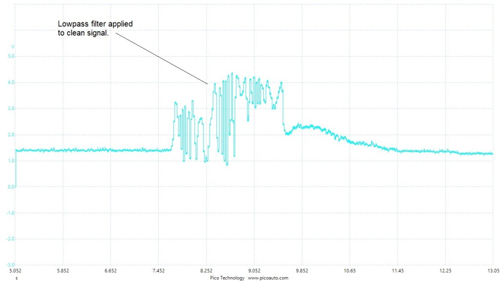
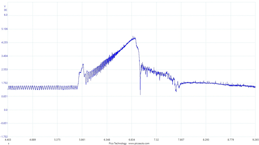
This is the same signal, but using the scope’s maths channel, I have produced a cleaner signal.

This image shows the same engine MAF signal, with a new good quality sensor fitted to it.
As you can see, the maximum output is still at 4.3 volts, but now the signal is a smooth linear waveform.

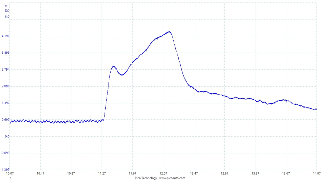
What a difference a good sensor makes.
This sensor, not only improved or corrected the slight hesitation in acceleration, but sorted out the fuel trim issue that was present before.

This next image comes from a turbo charged petrol engine MAF.

As before, this capture was taken with the engine idling to wide open throttle and back.

This is another sample to illustrate how each capture may differ slightly.

The following waveform shows the same type of MAF only from a diesel turbo engine vehicle.

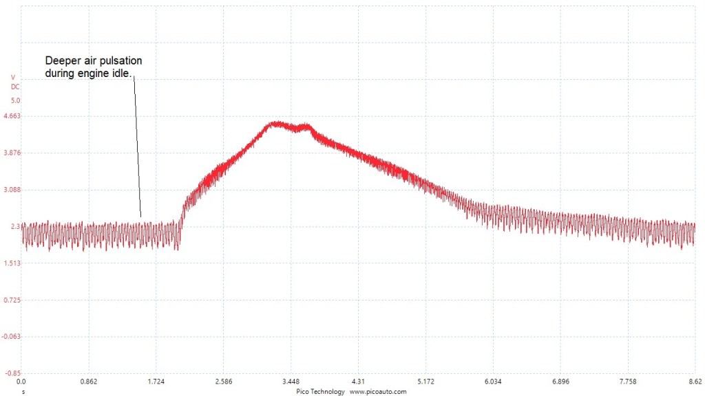
You can see how the profile is much less aggressive than with the petrol engine MAF. This is due to the absence of a throttle butterfly and so there is no sudden air movement. Also you will notice, that generally, the air pulsations are deeper during the no load condition at idle. Another diesel engine characteristic.

If we add in another channel, showing the accelerator pedal, we get better idea of progressive increase and decrease in air flow.

The sensors shown so far have all been ‘hot film’ sensors, with an analogue signal. The following are ‘hot film’ digital sensors. These have a frequency response proportional to output and it becomes a challenge to evaluate them, as there are so many variations of design.

As you will see in the following samples, unlike the analogue signal MAF’s, you cannot apply a ‘rule of thumb’ approach to diagnosing MAF integrity. The signals vary so much from manufacturer to manufacturer and even from the same manufacturer.

The first image I have, was taken from a diesel turbo direct injection system using a Hitachi digital MAF.

As you can see, there is very little useful information in this capture, other than there is a voltage present.

This MAF produces a frequency output with a relatively fixed duty cycle, as you will see in the following image.

I say relatively, because the duty cycle can be seen to change slightly during a wide open throttle event, but there is no mention of duty in the technical specifications for this specific MAF sensor and duty cycle very often changes with frequency unless very specifically controlled.

Using the facility built in to the Pico software I have used a 2^nd channel with a specific coupling utility for frequency. This is not possible on all scopes.

As you can now see, this image is much more useful.

The sample below is from a Bosch HFM digital sensor.

With the aid of the software again, a more useful sample is illustrated.

The no airflow figure for this was recorded as 1.8kHz. I don’t have specification for maximum airflow, but I’m guessing it’s close to 5kHz.

Now in this next set of waveforms you will see another version of the digital sensor and this one is quite unusual in its design.

It comes from a common rail diesel direct injection Bosch injection system.

I have shown this part of the signal, which was captured during normal engine idle, as it illustrates the unique signal the MAF produces. I show this because it confused me at first, but in reality it is just the same as the others. Here is a close up of the above.

When I first saw this pattern, I thought there was a particular significance in the high frequency cycling in the signal. In fact it is the normal idling airflow pulses that occur, only with this MAF the signal looks odd. The other thing with this MAF is, that most digital MAF sensors produce a higher frequency for higher airflow.

Lets have a look at this signal as it passes into a wide open throttle snap. I’ll only show the frequency signal.

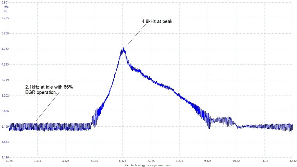
Maximum airflow specification is 1kHz. The maximum airflow reading here was captured at 960Hz.
No airflow specification is 5kHz. The no airflow reading captured here was 4.97kHz.
Natural idle figure captured was approximately 1.9kHz

For this capture I used a feature of ‘Bandwidth limiting’. This is a feature where you can restrict the bandwidth of the signal you are going to measure. As I knew the maximum frequency for this sensor is 5kHz, a restriction to 20kHz is perfectly OK and allows for a much cleaner signal acquisition. I also used the sensor ground to help improve the signal noise.

For some reason, with these sensors, the signals are very noisy with high frequency and I know there was no problem with this sensor. The non restricted capture is really messy.

This is a useful feature of some scopes. Watch out for this feature, but be careful with it, as you may miss something that is actually a fault.

Manifold Absolute Pressure sensors.

In this next set of images, we’ll look at Manifold Absolute Pressure (MAP) sensors.

These sensors measure, as there name suggests, absolute pressure. This means they measure the atmospheric pressure, when the engine is switched off and any measurement is above or below this reading. Typically, in the motor trade, the pressure in the inlet manifold of a petrol engine is referred to as ‘vacuum’. If you were measuring the ‘vacuum’ with a conventional ‘vacuum gauge’ you would expect to see a little over ½ bar of vacuum. However, in reality, you are measuring a positive pressure, just less than atmospheric. So atmospheric pressure is typically around 1000 millibar and so a petrol engine idling should be running at about 300 to 400 millibar. (Just rough figures you understand).

This first image, is taken from a 4 cylinder petrol engine.

The next image shows a MAP signal during start-up. I’ve included the ignition trigger signal, to represent engine status.

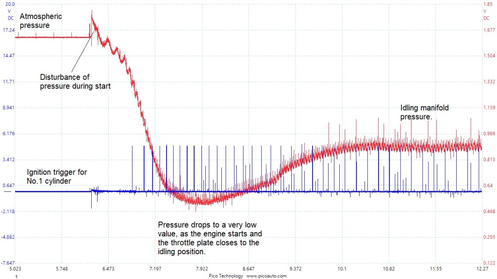
You can see, from the next image, how the pressure signal can show you engine operation details.

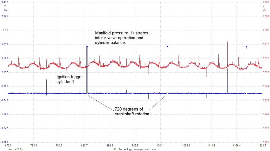
Using the next image, you can see how useful a good MAP signal can be.

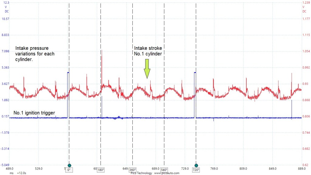
You can see that the peak value of the MAP signal, represents approximate top dead centre (TDC) for the piston. This is approximate, as it shows a potential stall in air flow due to the intake valves being closed during the compression stroke. Additionally, the trough value should be approximate bottom dead centre (BDC) of the intake stroke, as the piston cannot pull the air anymore.

The following image shows a wide open throttle (WOT) burst, as in the first image. It shows how the manifold pressure rises to atmospheric pressure as the throttle butterfly opens. These images have all come from naturally aspirated engines.

This last image is from a turbo charged engine.

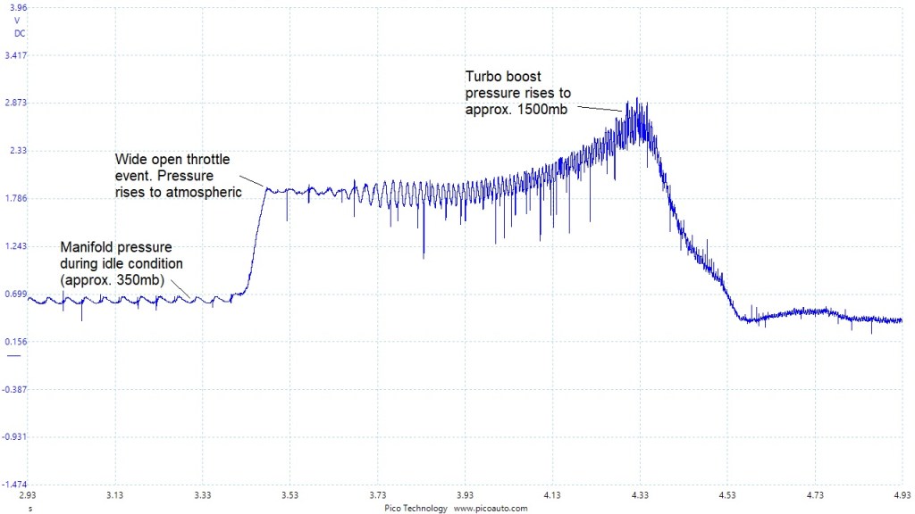
You can see the difference between the naturally aspirated MAP signal and the turbo charged signal.

Crankshaft sensors.

These sensors can be inductive analogue sensors, which produce there own current or digital Hall effect’ sensors, which use a power and ground, along with a signal.

The first type of sensor I will show, is the common ‘Inductive’ sensor. Meaning the sensor produces a voltage as a result of magnetic inductance. Typically these are 2 wire sensors, but early versions usually had 3 wires, the 3^rd being a screening circuit for the COAX type wiring.

The sensor shown here, only has 2 wires, which are twisted for interference suppression.

I have captured this using a common ground connection, (at the negative of the battery), and this sensor is a ‘floating ground’ sensor. The pattern is fine, but the amplitude is not accurate.

I talked about ‘floating ground’ sensors earlier in the guide. In the next image I will show you what it means in the case of an inductive sensor with a floating ground circuit.

This image is taken from the same sensor, only using 2 channels of the scope, to measure both pins of the sensor.

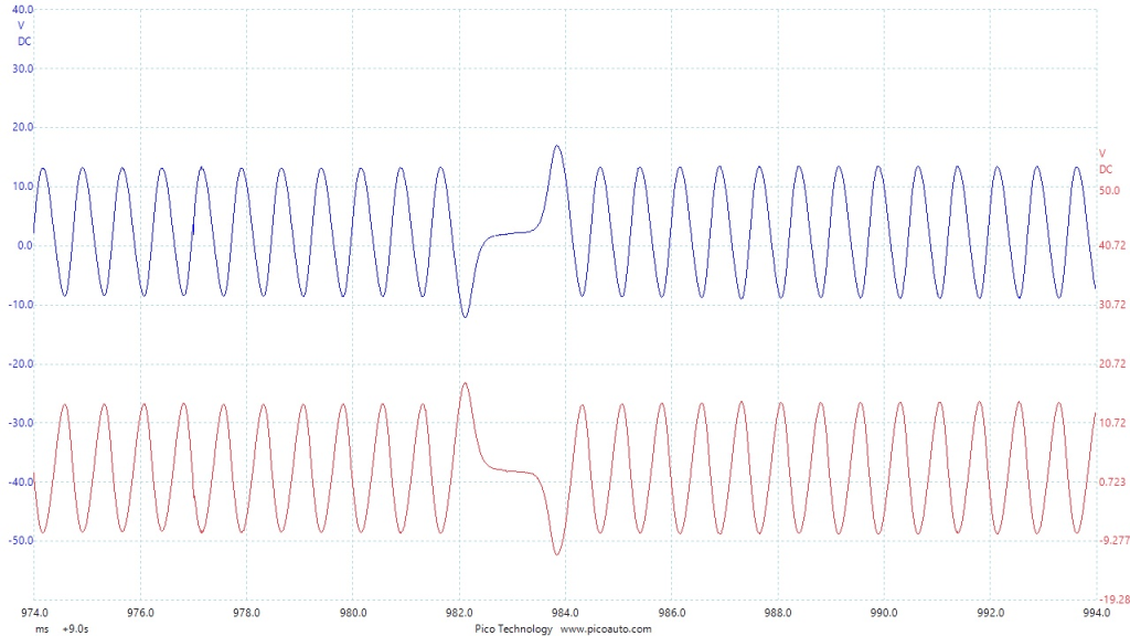
You can see how the negative side of the sensor, (in this case the red channel), is a mirror image of the positive side. Not all inductive sensors use a floating ground circuit, so always be aware.

With this sensor I did take a sample of the full amplitude, by connecting channel A across the sensor, meaning the scope channel ground was connected to pin 2 of the sensor, instead of the common ground at the battery negative terminal, as before.

Take a look at the capture and look at the voltage scales.

I also took an image to illustrate the difference.

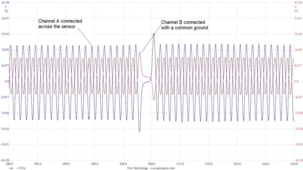
You maybe wondering why the red channel is not in the centre of the blue channel, even although the 0 volt markers, either side, are in the same horizontal plain.
We’ll see the reason for this anomaly, in the next image.

I have placed cursors at the 0 volt markers and a cursor at the centre line of the red channel waveform.

Channel A (Blue): differential connection across the sensor.
Channel B (Red): common ground connection.

The bias voltage is not visible with a differential connection. It is what the control unit uses to determine circuit integrity.

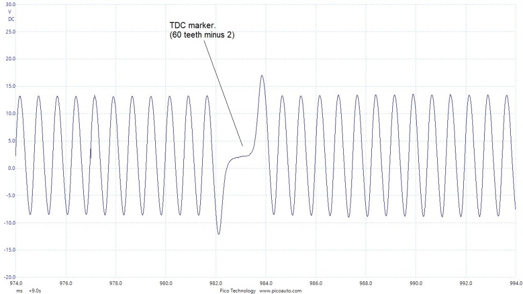
This final image just illustrates the full revolution of the crankshaft, so that you can see the 60 teeth minus 2 teeth.

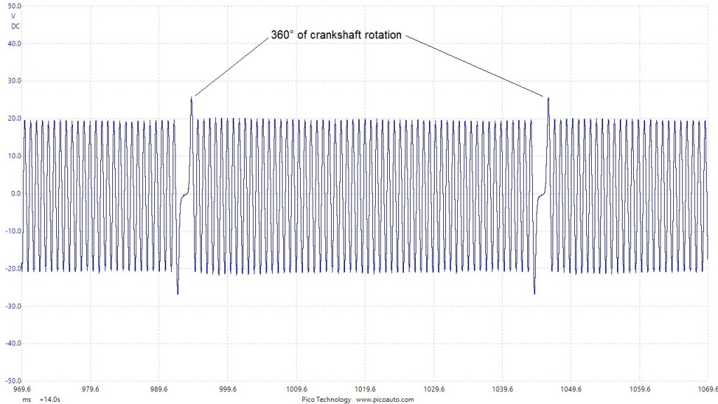
Inductive engine speed or crankshaft sensors have been around for a long time and they don’t all look like the signal I have shown. So, as with most scope analysis, always look for repeating patterns.

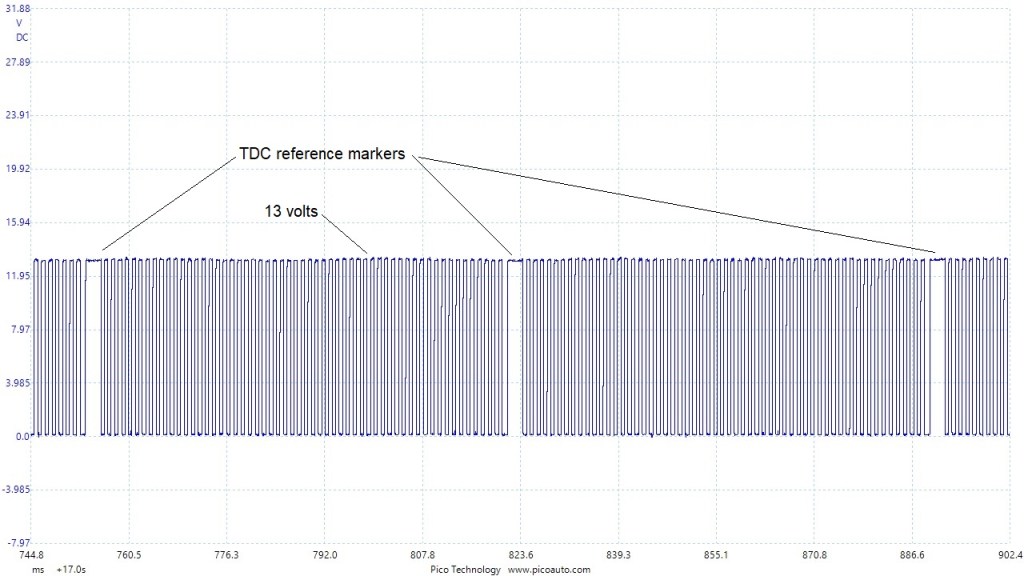
This is taken from a Subaru H6 non start, during cranking.

This next one is from 1987 Porsche 911 and has a speed sensor and a TDC reference sensor.

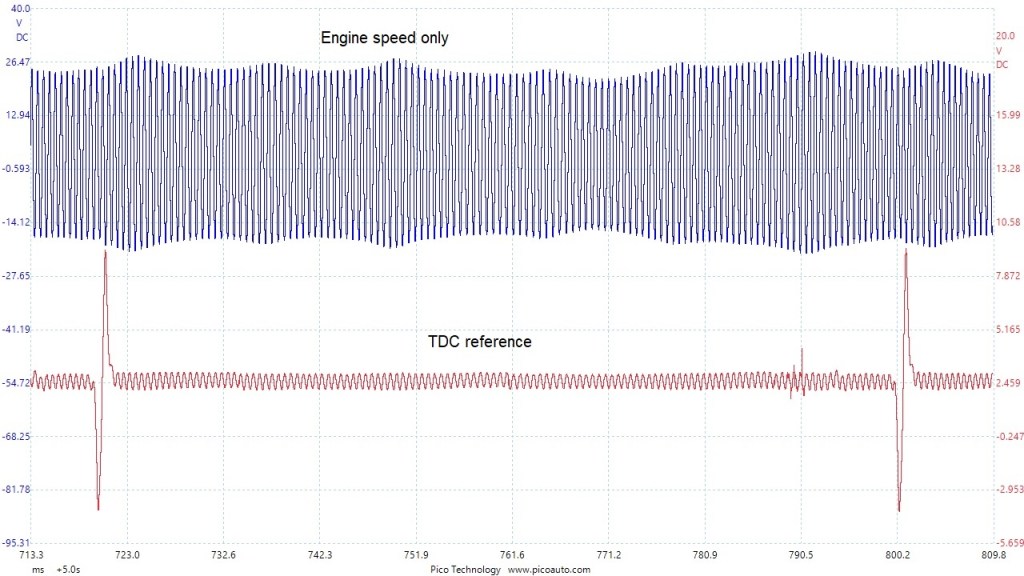
This represents early engine management in the form of ‘Bosch Motronic’.

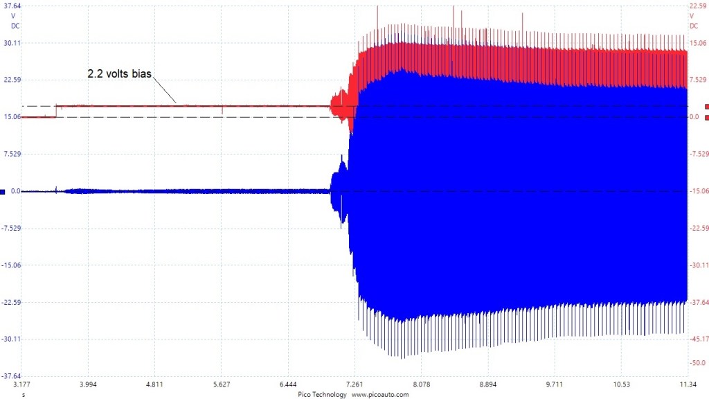
This is the last of my inductive sensor images. I have included it as it shows a common failure in operation.

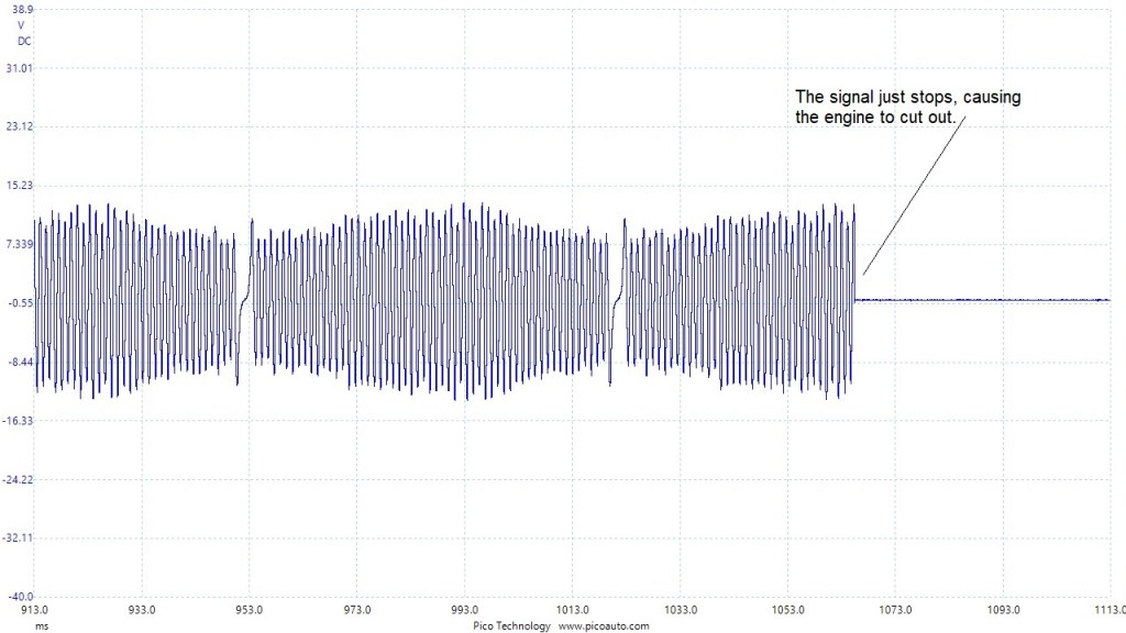
As the engine heats up, the sensor windings heat up and go open circuit. When the sensor cools down, it returns operation and the engine is able to start again.

In the next set of images, we’ll look at ‘digital’ crankshaft sensors. As time moves on, these sensor have become far more utilised. These are all ‘Hall Effect’ sensors and so require a power supply, a ground and a signal circuit.

Take a look at this common petrol engine crankshaft sensor signal.

This sensor uses a 5 volt supply, a ground and, as you can see, a battery voltage signal. Not all digital sensors have this configuration, as you will see, but I thought it useful to point this out, from the off.

In the following image, you will see a common 5 volt signal ‘Hall effect’ sensor. Again it is powered by 5 volts, with 0 volt ground reference, but in this case the signal is 0 to 5 volt.

When analysing these sensors you need to look at the profile of the signal, including the high and low voltages. Look at how close to zero the low voltage is, as this is often a sign of a bad sensor. As with all these signals, compare to a known good one.

I have shown two significant signal voltage ranges, for crankshaft sensors. Battery voltage in the first signal and a logical 5 volt in the second. I have many variations of voltage levels in my library of samples, so always compare to known good samples before condemning a sensor on voltage range alone.

I will show one more crankshaft sensor signal configuration. But remember there can be several different signals used on many different vehicles.

Camshaft sensors

Now we’ll take a look at the crankshaft sensor’s cousin; the camshaft sensor.

I won’t go too much into these for the simple reason, they’re exactly the same as the crankshaft sensor. They come in inductive and hall effect, with many different pattern configurations.

Their use is more about identification of particular cylinders.

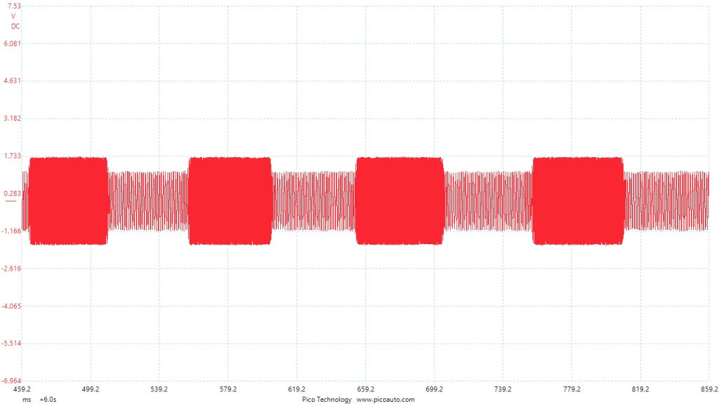
We’ll have a look at the ‘AC’ excited sensor. It is basically a dual field inductive sensor, which is powered with an ‘AC’ signal on both fields. When the sensor field is interrupted by a ferrous target, the signal’s phase shifts.

This first image was sampled by using a differential connection, for ease and clarity.

I’ll try and show you a bit more detail on how they work. I don’t see them fitted on vehicles later than the early 2000’s, but who knows!

The technology is still used, as I have seen it used for travel indication sensors, such as Clutch travel, because they can be housed in harsh environments.

This image was taken from a Vauxhall Vectra and I used one channel for each phase.
The section displayed is the transition phase as the camshaft pulley rotates the target block past the sensor.

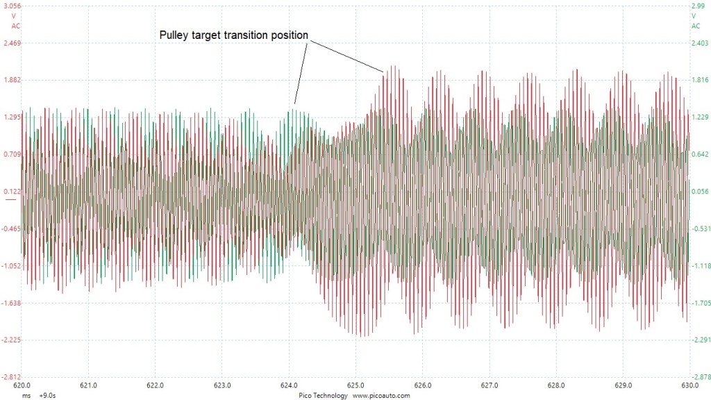
You can see the phase position shifts over during the transition with the target. It clearly effects the amplitude of the red channel also.

Look at the position between the red channel and the green channel. The red channel phase has shifted to the right. The frequency of the signals has not changed, just their relationship.

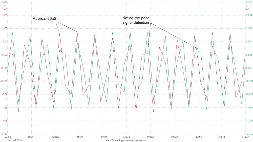
Speaking of frequency. This sensor runs at a very high frequency, approximately 17kHz. I only mention it, because the next image illustrates the sampling restrictions on the scope capture.

I captured it using a 2 sec/div setting, giving me 20 seconds of screen time, but I left the scope sampling rate at the standard default 1 mega-sample. That setting is normally fine for a good zoom function, when looking at cam and crank sensors and I only wanted to see the operation.

Now take a look at the lack of detail, when the zoom function has magnified the sample by about 25 times.

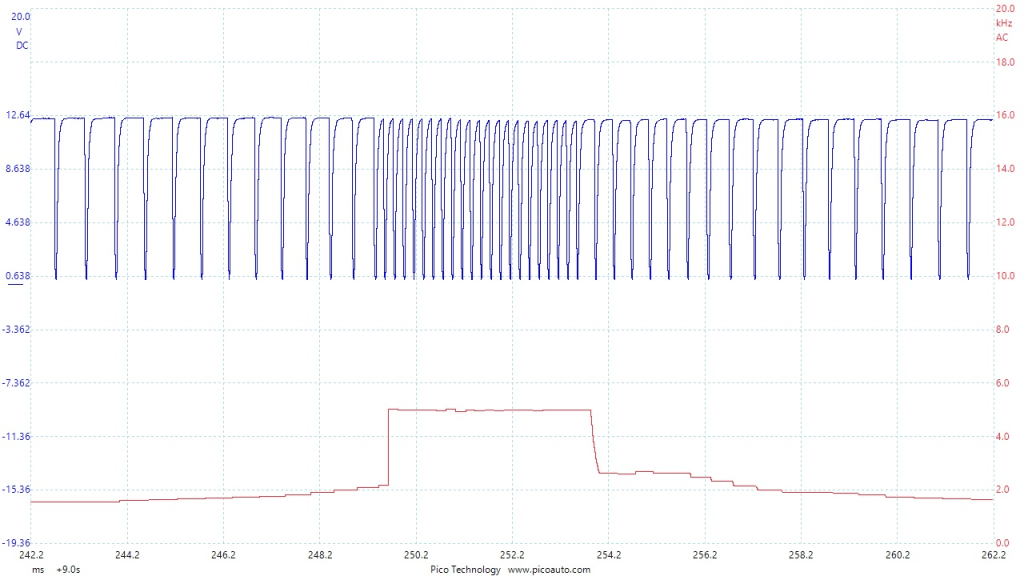
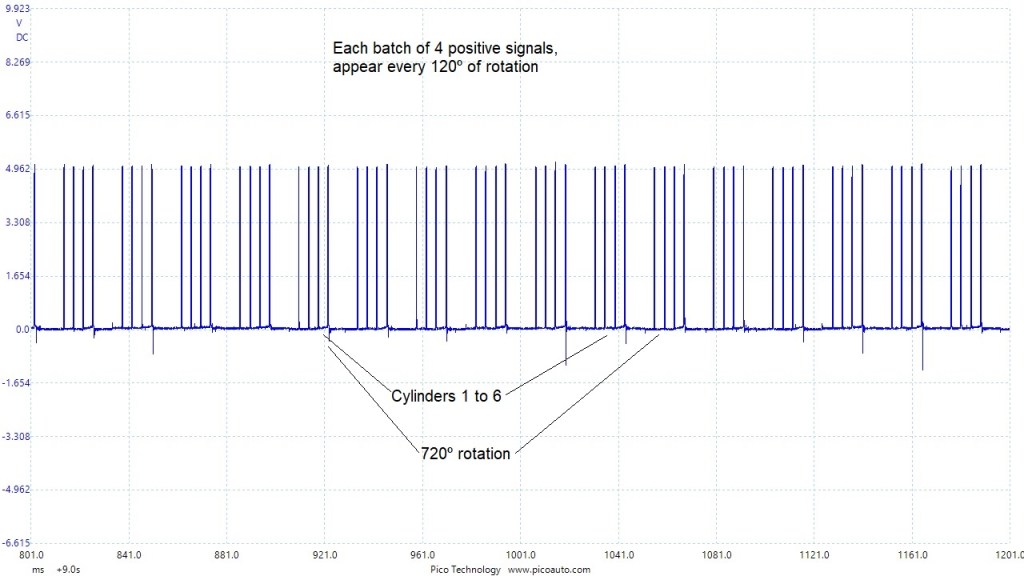
Hall effect sensors became the more common choice as the years advanced. I have chosen this one to show, as it easily portrays the cylinder identification method. It comes from a 4 cylinder Nissan engine with a firing order of 1,3,4,2.

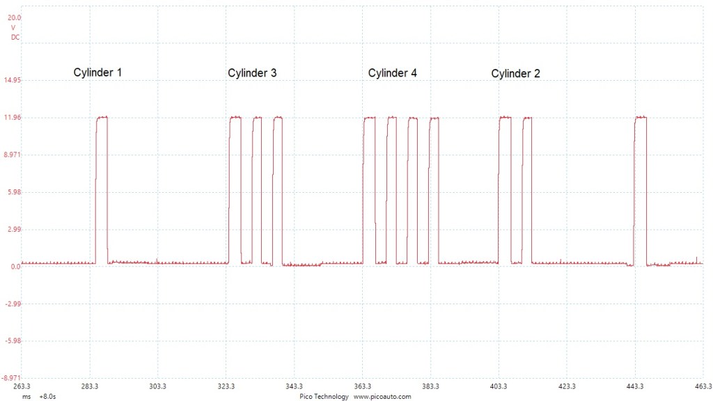
The sensor shown above, as you can see, uses an approximate 12 volt pull down signal. I find you don’t see too many signals that represent cylinder numbers, so clearly. The computer only needs to recognise a pattern in conjunction with a firing event. Mostly I find the sensors to use a 5 volt signal nowadays.

Accelerator Pedal sensor or Throttle Position sensors

Input sensors such as accelerator pedal position and throttle position can prove to be an interesting subject, as once again, they have evolved somewhat.

They started life as a Throttle Switch. The more sophisticated being a three position switch, as fitted to early electronic injection systems like Bosch LE2. The switch would notify the control unit of the idle position, the mid travel position and the full throttle position.

Sadly I don’t have a scope capture of this type to demonstrate.

These switches were replaced with the more common single channel ‘Throttle POT’, that is to say, throttle position sensor. These remained common until electronic throttle butterfly units came into play.

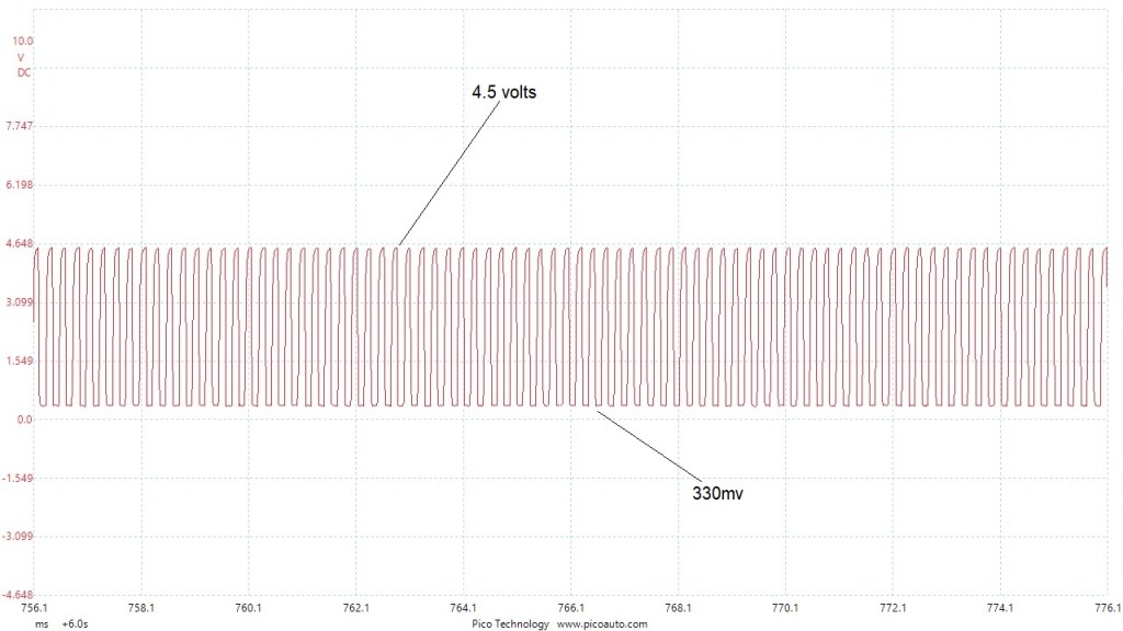
This image, illustrates a fairly common 3 pin Throttle Position Sensor (TPS).

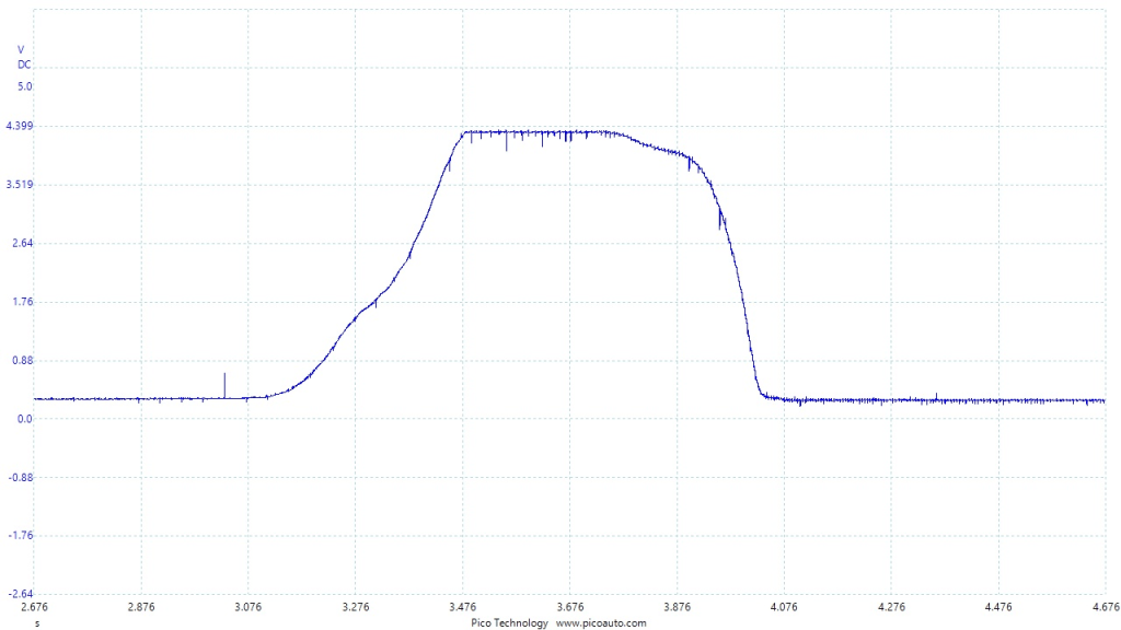
The idle position reports approximately 0.3 volts and the full throttle position reports about 4.3 volts.

Any voltage below the 0.3 volts would generally mean ‘short circuit’ and any reading above 4.3 volts would mean ‘open circuit’. Although they might not be accurate values, but that was the general principle. The first generation TPS’s in my memory used 0.5 volts as idle and 4.5 volts as full throttle, meaning anything below 0.5 and above 4.5 was a fault.

Those values have definitely changed over the years. Always try and find service information for fault code setting criteria.

The simple single channel TPS was used in conjunction with injection management systems, which would also utilise various load sensors, such as manifold absolute pressure and airflow or airmass meters.

The following images come from a single point or mono point injection body system. Very basic in operation with no external load sensing capabilities. As a consequence, the TPS had to be more reliable. This was the first system I ever come across, with a dual track TPS.

You can see in the above image, the two tracks respond differently. The blue channel, which sits at 0.3 volts for idle and rises to 4.9 volts for WOT. The red channel rises from 0.02 volts, at idle, to 4.4 volts WOT.

You will also notice that the blue channel is rapid to rise, or course, and the red channel is slower or finer to rise.

This is what the ECM uses to compare for reliability.

In the next image of the same system, you will notice a fault. This was quite a common failure of these TPS units. Take a look.

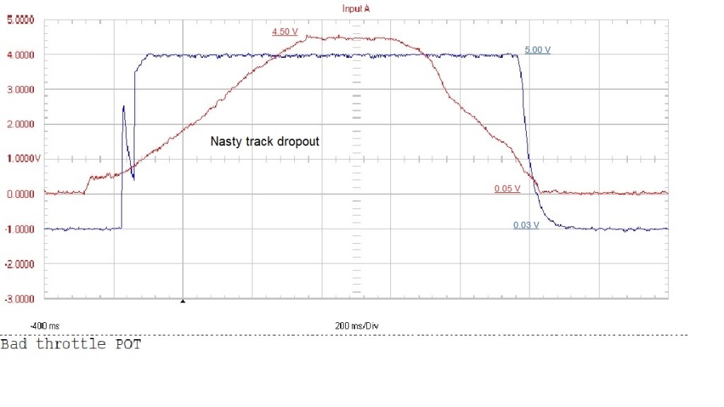
The results of this condition was a fairly noticeable hesitation. There were rarely any fault codes recorded, unless you were lucky and live data was non-existent, as I remember. Sometimes you could pick this fault up using a good DVM, as indeed I did manage many times.

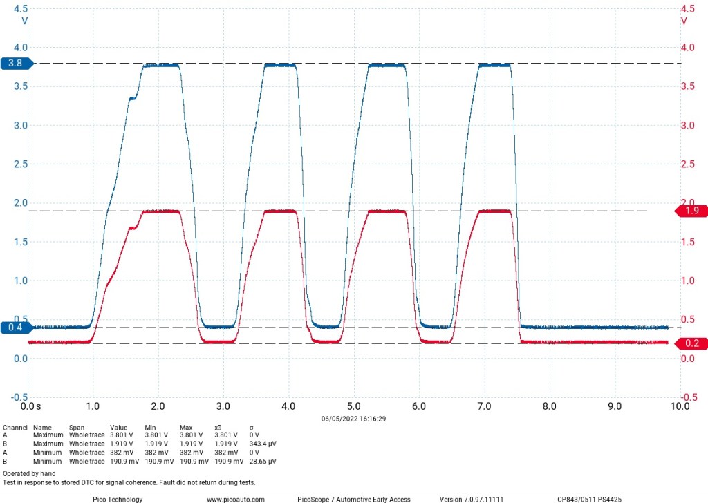
The following image shows a very common set-up of an accelerator pedal sensor with two tracks. One track is exactly half the value of the other.

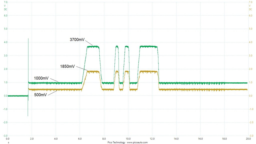
That image came from a Vauxhall Astra, but it is a very common sample. Typically the ECM will measure the difference between the two signals to verify the operation. The sensor has six terminals, two 5 volt references, two signal ground references and two proportional signals. Always a good idea to check all terminals, especially if one of the position signals are incorrect.

The image below, was taken from a 2002 Peugeot 607 HDi. It is a commonly used remote 2 track pedal sensor.

For analysis, I have filtered the image to 30kHz.